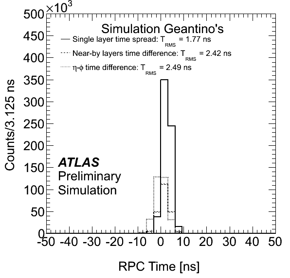
The plot shows the RPC cluster hit time spread for both views of a layer (corrected by signal propagation along strip) and the relative time spread between near-by layers for the same view (not corrected by signal propagation along strip) and between the two views of the same layer (corrected by signal propagation along strip). The RPC cluster hit time is defined as the minimum time of adjacent hits. The data correspond to simulated event generated by Geantino particles (neutral and not interacting particles which leave hits in the active volumes).
eps png
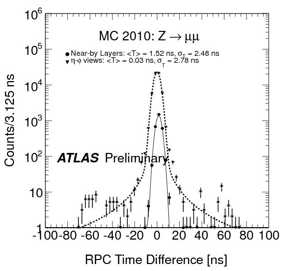
The plot shows the RPC cluster hit time spread: between near-by layers for the same view (not corrected by signal propagation along strip), between the two views of the same layer (corrected by signal propagation along strip). The RPC cluster hit time is defined as the minimum time of adjacent hits. The data correspond to simulated Zmumu events and the RPC cluster matched to CM muons (deta,dphi<0.1). The superimposed fits are made with a Gaussian function (central core) for the near-by layers and same view. For the two views of the same layer a symmetric power law function with exponent equal 5 (non-Gaussian tails) is added. The indicated average time and spread time correspond to the Gaussian core.
eps png
The plot shows the RPC cluster hit time spread in pp 7 TeV 2011 data between near-by layers for the same view (not corrected by signal propagation along strip) before and after off-line time calibration. The RPC cluster considered are matched to CM muons (deta,dphi<0.1). The RPC cluster hit time is defined as the minimum time of adjacent hits. The superimposed fits are made with a Gaussian function (central core) and symmetric power law function (non-Gaussian tails). The indicated average time and spread time correspond to the Gaussian core. The data correspond to a run of period G and Muon_Physics stream when detector and beam flags were green.
eps png

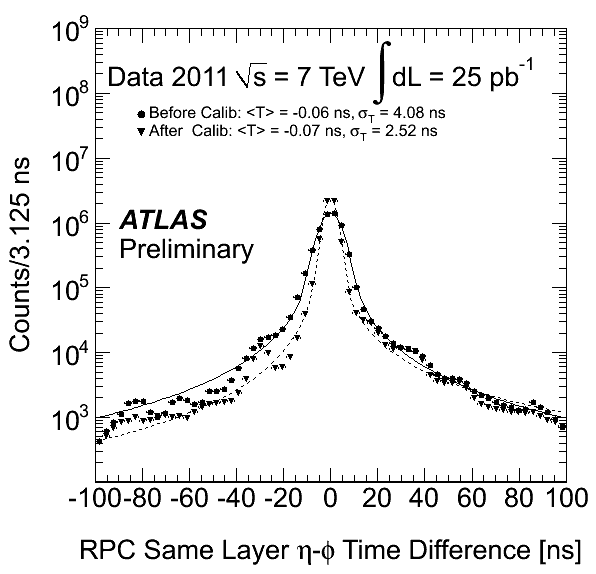
The plot shows the RPC cluster hit time spread in pp 7 TeV 2011 data between views of the same layer (corrected by signal propagation along strip) before and after off-line time calibration. The RPC cluster considered are matched to CM muons (deta,dphi<0.1). The RPC cluster hit time is defined as the minimum time of adjacent hits. The superimposed fits are made with a Gaussian function (central core) and symmetric power law function (non-Gaussian tails). The indicated average time and spread time correspond to the Gaussian core. The data correspond to a run of period G and Muon_Physics stream when detector and beam flags were green.
eps png
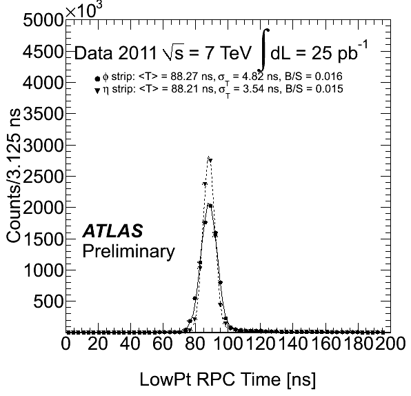
The plot shows the RPC cluster hit time spread in pp 7 TeV data for LowPt layers and both views (corrected by signal propagation along strip). The RPC cluster considered are matched to CM muons (deta,dphi<0.1). The RPC cluster hit time is defined as the minimum time of adjacent hits. The superimposed fits are made with a Gaussian function (central core) and asymmetric power law function (non-Gaussian tails). The indicated average time and spread time correspond to the Gaussian core. The ratio of background events inside a +/-3sigma window and the signal events in the Gaussian core is also indicated. The data correspond to a run of period G and Muon_Physics stream when detector and beam flags were green.
eps png
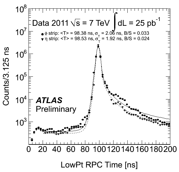
The plot shows the RPC cluster hit time spread in pp 7 TeV data for LowPt layers and both views (corrected by signal propagation along strip) after off-line calibrations. The RPC cluster considered are matched to CM muons (deta,dphi<0.1). The RPC cluster hit time is defined as the minimum time of adjacent hits. The superimposed fits are made with a Gaussian function (central core) and asymmetric power law function (non-Gaussian tails). The indicated average time and spread time correspond to the Gaussian core. The ratio of background events inside a +/-3sigma window and the signal events in the Gaussian core is also indicated. The data correspond to a run of period G and Muon_Physics stream when detector and beam flags were green.
eps png
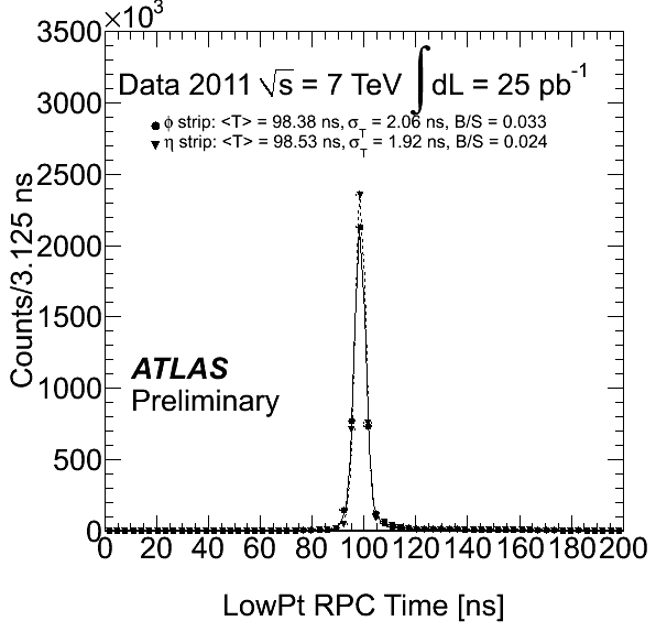
The plot shows the RPC cluster hit time spread in pp 7 TeV data for LowPt layers and both views (corrected by signal propagation along strip) after off-line calibrations. The RPC cluster considered are matched to CM muons (deta,dphi<0.1). The RPC cluster hit time is defined as the minimum time of adjacent hits. The superimposed fits are made with a Gaussian function (central core) and asymmetric power law function (non-Gaussian tails). The indicated average time and spread time correspond to the Gaussian core. The ratio of background events inside a +/-3sigma window and the signal events in the Gaussian core is also indicated. The data correspond to a run of period G and Muon_Physics stream when detector and beam flags were green.
eps png
The plot shows the RPC cluster hit time spread in pp 7 TeV data for HighPt layers and both views (corrected by signal propagation along strip) after off-line calibrations. The RPC cluster considered are matched to CM muons (deta,dphi<0.1). The RPC cluster hit time is defined as the minimum time of adjacent hits. The superimposed fits are made with a Gaussian function (central core) and asymmetric power law function (non-Gaussian tails). The indicated average time and spread time correspond to the Gaussian core. The ratio of background events inside a +/-3sigma window and the signal events in the Gaussian core is also indicated. The data correspond to a run of period G and Muon_Physics 8 stream when detector and beam flags were green.
eps png

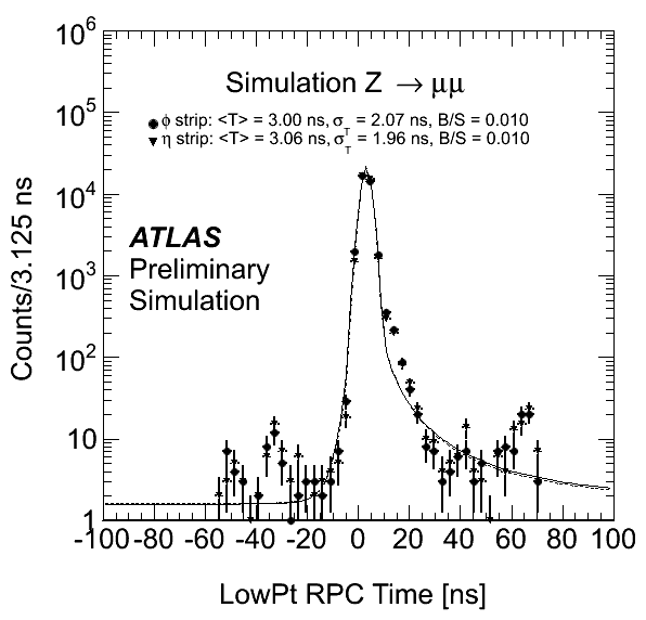
The plot shows the RPC cluster hit time spread in simulated Zmumu events for LowPt layers and both views (corrected by signal propagation along strip). The RPC cluster considered are matched to CM muons (deta,dphi<0.1). The RPC cluster hit time is defined as the minimum time of adjacent hits. The superimposed fits are made with a Gaussian function (central core) and asymmetric power law function (non-Gaussian tails). The indicated average time and spread time correspond to the Gaussian core. The ratio of background events inside a +/-3sigma window and the signal events in the Gaussian core is also indicated.
eps png
The plot shows the measured particle velocity distribution of relativistic particles from the IP with and without IP constrain in the fit. The velocity without IP constrain is extracted from a linear fit to the incremental distance from the ideal IP (0,0,0) of 6 ordered space points, obtained averaging RPC eta-phi clusters matched with CB tracks (deta,dphi<0.1) on each of 6 RPC layers, versus 6 times, obtained by averaging all RPC eta and phi cluster time defining the associated space point after signal strip propagation, subtracting 5 ns and adding the expected TOF. The velocity with IP constrain is obtained adding the point d=0 and t=0 with errors equal to 1 cm and 1 ns respectively. The data correspond to simulated event generated by Geantino particles (neutral and not10 interaction particles which leave hits in the active volumes) without IP spread.
eps png

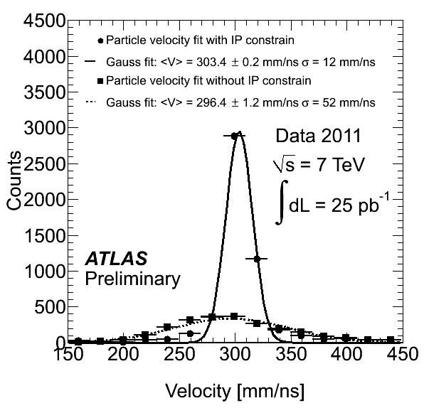
The plot shows the measured particle velocity distribution of relativistic particles from the IP with and without IP constrain in the fit in pp 7 TeV data. The velocity without IP constrain is extracted from a linear fit to the incremental distance from the ideal IP (0,0,0) of 6 ordered space points, obtained averaging RPC eta-phi clusters matched with CB tracks (deta,dphi<0.1) on each of 6 RPC layers, versus 6 times, obtained by averaging all RPC eta and phi cluster time defining the associated space point after signal strip propagation, off-line calibration, subtracting 100 ns and adding the expected TOF. The velocity with IP constrain is obtained adding the point d=0 and t=100 with errors equal to 1 cm and 1 ns respectively. The data correspond to a run of period G and Muon_Physics stream when detector and beam flags were green.
eps png
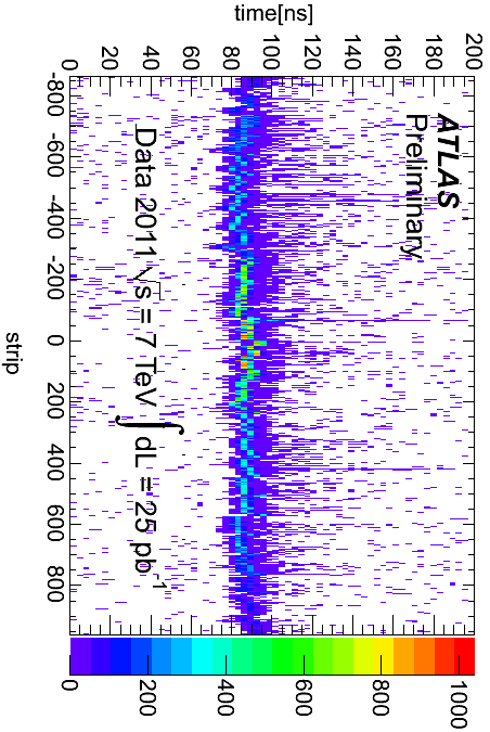
The plot shows the RPC cluster hit time (corrected by signal propagation along strip) vs strip number for one RPC layer from side C to side A in pp 7 TeV before off-line calibration. The RPC cluster considered are matched to CM muons (deta,dphi<0.1). The RPC cluster hit time is defined as the minimum time of adjacent hits. The data correspond to a run of period G and Muon_Physics stream when detector and beam flags were green.
eps png
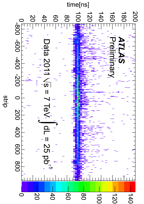
The plot shows the RPC cluster hit time (corrected by signal propagation along strip) vs strip number for one RPC layer from side C to side A in pp 7 TeV after off-line calibration. The RPC cluster considered are matched to CM muons (deta,dphi<0.1). The RPC cluster hit time is defined as the minimum time of adjacent hits. The data correspond to a run of period G and Muon_Physics stream when detector and beam flags were green.
eps png
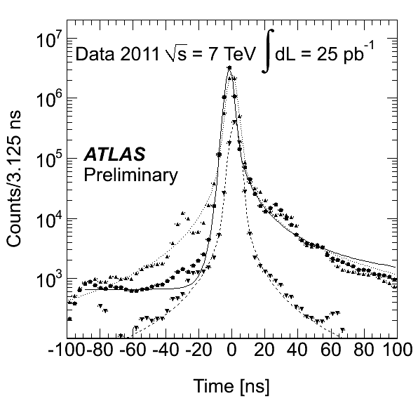
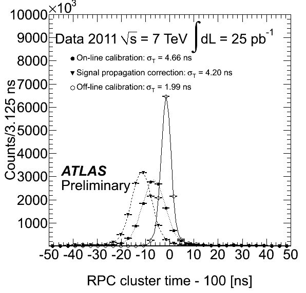
The plot shows the distribution of the time of the RPC clusters in 2011, after subtraction of a common offset of 100 ns corresponding to one half of the readout window size. The data sample used is the muon stream where events are selected requesting good detector quality and beam conditions. The different distributions refer to the time as available in the raw data, after the on-line time calibration applied at the level of readout and trigger electronics (solid circles), to the time after the correction for the delay due to the signal propagation along the strip (solid triangles) and to the time after correction for signal propagation and after off-line time calibration (empty circles).
eps png
The plot shows the distribution of the time of the RPC clusters (solid dots) in 2011, after subtraction of a common offset of 100 ns corresponding to one half of the readout window size and after full offline calibration (correcting for signal propagation time and off-line time equalization), the distribution of the difference in time between RPC clusters in two near-by gas volumes and same view (down triangle), the distribution of the difference in time between RPC clusters in the readout panels reading the orthogonal views of a single gas volume after correction of each view for the delay related to the signal propagation along the strip (up triangles). The superimposed fits are made with a Gaussian function, describing the core of the distribution, and an asymmetric power law function for the non-Gaussian tails. The fraction of events in the tails underneath the gaussian component in an interval of +/-3 sigma is about 2.5% for the cluster time distribution and the difference in time between nearby gas-gaps and below 0.5% for the difference in time between two views of a single gas-gap. The data sample used is the muon stream where events are selected requesting good detector quality and beam conditions.
eps png